Github

Introduction

This website represents the final presentation of the work that our team has done attending the course of “Didactic Laboratory of Information Engineering” held by Dr Riccardo Bernardini in the Master degree of Electronic Engineering at the University of Udine.  The aim of this course is to provide the students the skill to work in a team starting with the analysis of a problem and ending up with a solution.

In our specific case, the task is to project headphones able to let the user hear the voices around him and that filter out loud and brief noise that could damage its hearing. Thinking about real life, it’s quite obvious that there is a wide number of applications of such a product, like for instance, the military field where the shot of a gun could cause deafness.

 In the TRL scale, we stopped at the fourth level of project meaning that we have tested our device only in a laboratory, trying as fast as possible to speed up a process that would require years to be finished in all its details in a modern industry. 

Getting Started

Like every reasonable project, the starting point consists in reading a lot of papers in order to increase the “know how” of the group and realize the solutions that are already present in literature. In our specific case we had the opportunity to see that there are two main families of 
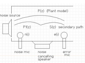
solutions: digital and analogical, respectively. In both cases the aim is to generate a wave that must delete the noise (like in the figure) obtaining a null noise in the area near the ears.

 To understand analogic methodologies, we suggest to read carefully the sections [21], [22] and [23] listed in the bibliography. From those papers we understand that even if analogic world is cheaper, it’s not an accurate solution. This is mainly because the circuitry must have minimum errors on gain and phase in order to guarantee the stability of the system. Moreover, this solution is not robust if we change the environment or the temperature that surrounds us. Another problem is that we need to know exactly the transfer function of the system that is due to the ear’s auricle of the user.

Among all the famous algorithms that are employed in Active Noise Reduction (ANR) we find FXLMS and FXLMM (see [26] in bibliography). In particular, this last one is the most efficient and stable one for impulsive noise.

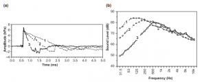
Active filters for noise reduction are much more efficient to reduce noise at high frequency, while instead for low frequencies it’s better to choose properly the transmission medium crossed by the noise before getting to the hearing channel.

To look deeper inside the ANR theory, look at the papers in [26],[36] and [37].

The Gunshot

Without getting too much in detail, if you wish to understand how to model a shot and the problems related to the environment afflicted by impulsive noise we suggest looking at [24] and [25].  It’s important to highlight that a shot can reach peaks up to 110 dB in a closed room and the typical behaviour is like the one shown in the figure. We can notice that it has a large band and this is a difficult thing to deal with because normal speakers with low output power cannot compensate it. 

The Headphones

The feedforward ANR system that we wish to implement is based on the scheme shown in figure and according to the simulations that are done in [32] and [34] it’s the most efficient against broadband noise like the one of a gunshot. 

Such a scheme leads us to model the system with a scheme made of blocs like the one in the lower picture. The source of the noise is the one we want to delete, and it’s read from the reference icrophone and we have the generation of a destructive wave through the speaker controlled by the
adaptive filter. Since the cancellation won’t be that perfect, we use a second microphone called “error mic” that is going to measure the residual noise near the hearing cavity, modifying the coefficients of the filter through a chosen algorithm that will make the system converge to zero.

The problems related to this solution are for sure:

  • The choice of the µ coefficient inside the algorithm that influences the convergence of the error
  • We must estimate Š following the procedure shown in [26],[35]·        

Despite that, through this solution we remove all the possible external noise. If we wish to let a voice pass, we just need to modify the system a little bit considering the need of digitalizing the voice oming
from a source, before broadcasting it via radio waves to the receiver’s headphones. Since this modification is quite simple to be done we won’t comment anymore on this step (for much details look at [8],[10] and [30]).

To reach top level performances, we must have S as flat as possible like shown in [31] and this is obtained positioning the error microphone in the point 8 of the last picture shown in this section. 

Causality Condition

Summing up, in the feedforward scheme we have all the following steps:

  • Measure the noise through the reference microphone and elaborate it
  • Compute the deleting wave
  • Broadcast the deleting wave and let it reach the error microphone

The time to make all these passages has to be smaller  compared to the time of propagation of the disturbing wave from the reference microphone to the error microphone. This is the so-called causality condition. Considering periodic disturbs it’s not necessary to respect this condition while in the case of non-periodicity we must deal with it, otherwise we would have attenuation problems. The time to compute the deleting wave could reach  worrisome values (even minutes) if we don’t respect randomness adding also instability to our problem. It’s pretty easy to understand that in our case the reference microphone should be at least a couple of meters far form the headphones ([38]), requiring a non-comfortable implementation and a too long convergence time. Once again, if randomness influences the convergency of the control filter it won’t influence at the same time the identification of the system (Kong and Kuo 1999).

Problems with the pratical implementation

  • The stability of the system strongly depends on the µ parameter choice inside the algorithm and on the input provided to the system.
  • The characterization and realization of ANR filters are too difficult with a low-level language, reason why we have preferred to study the problem more in general setting the right base for future development.
  • Risk of saturation for the microphone: if the shot is too peaked, we could damage the sensor.
  • The time to compute the filter’s coefficients is quite high: it could take almost 10 seconds, and this is something that the user would find annoying.
  • Causality condition not so easy to be implemented.
  • Impossible to reduce sounds that happen through “bone conduction”. This last phenomenon consists in an acoustic  wave that causes the vibration of the ear’s bones and consequently the propagation of a sound that reaches  our hearing without passing through the cavity. Our algorithm cannot take in account such an effect and to avoid this we suggest to use high cost materials such as the ones suggested in [21].
  • Processor with high computation power is required.

Because of all these problems and after having proved the low efficiency of ANR in the lab (look at simulation page) we have decided to leave behind this type of solution and instead to study algorithms that are for sure less efficient but easier to be implemented in the market and that require a lower computational cost. The new procedure is the following one:

  • Filter out all the sounds that are outside our headphones (either voices and gunshots)
  • Through a microphone that is positioned outside we choose properly the sounds to play through the speaker inside the headphones, removing the impulsive noise through the clipping method.

Clipping consists in playing the audio samples that are caught by the external microphone until when they are under a proper trigger threshold
chosen in a dynamic way, if the samples are over this level we have different ways to proceed:

  • ZERO CLIPPINGwe play null samples for the whole shot last
  • OLD CLIPPING: we repeat old samples to make the communication less annoying
  • COMPRESSION CLIPPING
  • Reconstruct samples that are removed by the clipping with INTERPOLATION: in particular,  we have identified two possible algorithms that lead to acceptable results that are, respectively the implementation of a polynomial function and the autoregression model (ARIMA) using samples before and after the shot ([18]).

The last solution is the most practical one and the only issue is due to the latency: it will take some time for the sound to arrive to the  hearing system because we need to process information in an electronic system. This last thing, by the way, can be solved in future choosing a processor without operating system and employing a smart programming language such as C.